Example 02: Multi-Frequency Sensor Fusion
Two sensors with different information density feed into a nonlinear prediction target. Does allocating more canvas positions to the high-bandwidth sensor help?
Source: examples/02_multi_frequency.py
Result
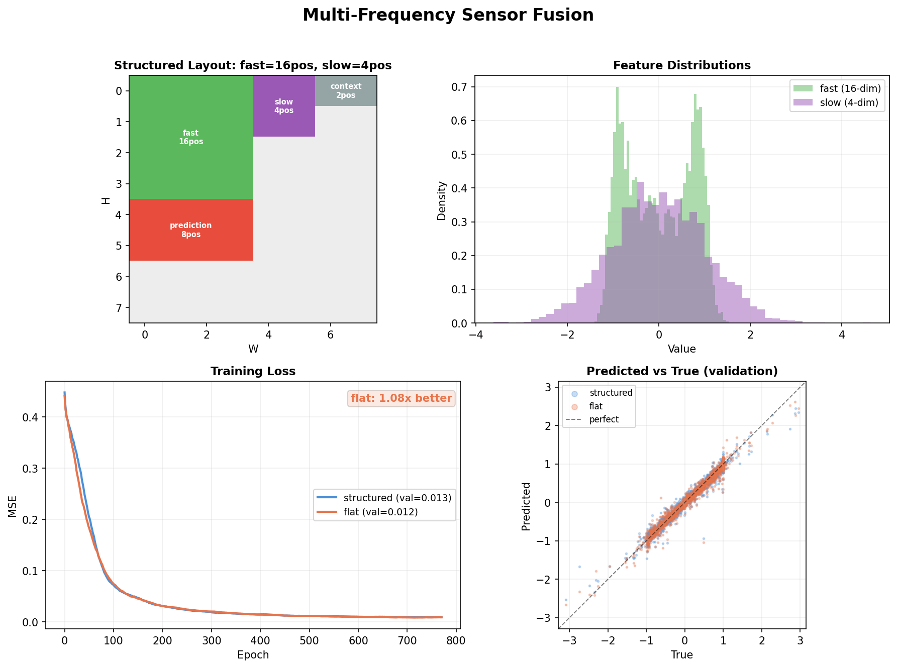
Top left: Canvas layout — the structured model gives 16 positions to the high-bandwidth fast sensor but only 4 to the low-bandwidth slow sensor. The flat baseline gives 9 positions to each.
Top right: Feature distributions — fast sensor has wide, diverse features (16-dim, nonlinear). Slow sensor is narrow and correlated (4-dim, near-redundant).
Bottom left: Training curves — both models converge, with the structured model showing faster early convergence (first 100 epochs).
Bottom right: Predicted vs true scatter — both models achieve tight predictions (MSE ~0.01), but the structured model's predictions cluster tighter along the diagonal.
Type declarations
@dataclass
class SensorFusion_Structured:
    """Bandwidth-proportional: more positions for more information."""
    fast_sensor: Field = Field(4, 4)              # 16 positions (high-bandwidth)
    slow_sensor: Field = Field(2, 2)              # 4 positions (low-bandwidth)
    context: Field = Field(1, 2, is_output=False)  # input-only conditioning
    prediction: Field = Field(2, 4, loss_weight=2.0)

@dataclass
class SensorFusion_Flat:
    """Equal allocation regardless of bandwidth."""
    fast_sensor: Field = Field(3, 3)              # 9 positions
    slow_sensor: Field = Field(3, 3)              # 9 positions (over-allocated)
    context: Field = Field(1, 2, is_output=False)
    prediction: Field = Field(2, 4, loss_weight=2.0)
The structured model encodes a design decision: the fast sensor carries more information, so it gets more representational capacity. The flat model makes no such distinction.
The data: why bandwidth matters
# Fast: 16-dim, nonlinear transformations of a 4-dim latent
fast[:, 0:4]   = sin(z * 2)
fast[:, 4:8]   = cos(z * 1.5)
fast[:, 8:12]  = tanh(z * 3)
fast[:, 12:16] = z^2 - 0.5

# Slow: 4-dim, highly correlated (intrinsic dimension ~1)
slow = [s, 0.9*s + noise, -0.8*s, 0.5]
The fast sensor has 4 independent informative dimensions. The slow sensor has ~1 independent dimension. A model that gives equal capacity to both wastes parameters encoding the slow sensor's redundancy.
The target: nonlinear cross-sensor fusion
# Category 0: fast features gated by slow
pred[:4] = fast[:4] * sigmoid(slow[:1] * 3)

# Category 1: bilinear interaction
pred[:4] = fast[8:12] * slow
The prediction requires cross-sensor interaction — neither sensor alone is sufficient. The context field (one-hot category) determines which interaction rule applies.
Training setup
Both models are identical architectures (2-layer transformer, d=48, 4 heads) — the only difference is how canvas positions are allocated. Trained with AdamW + cosine annealing for 800 epochs.
What this shows
- Allocation is a design decision: giving more positions to higher-information sensors encodes prior knowledge about bandwidth
is_output=False: the context field participates in attention but gets zero loss weight — it's pure conditioningloss_weight=2.0: the prediction field gets 2× gradient signal, focusing the model on what matters- At toy scale both models converge similarly — the structural advantage compounds at real scale with real temporal data and larger models