Example 03: CartPole Control

Behavioral cloning on a real gymnasium environment. Three models compared: flat MLP, canvas-structured BC, and canvas with self-consistency loss that creates feedback dynamics between predicted reward, done signal, and observation state.

Source: examples/03_cartpole_control.py

Result

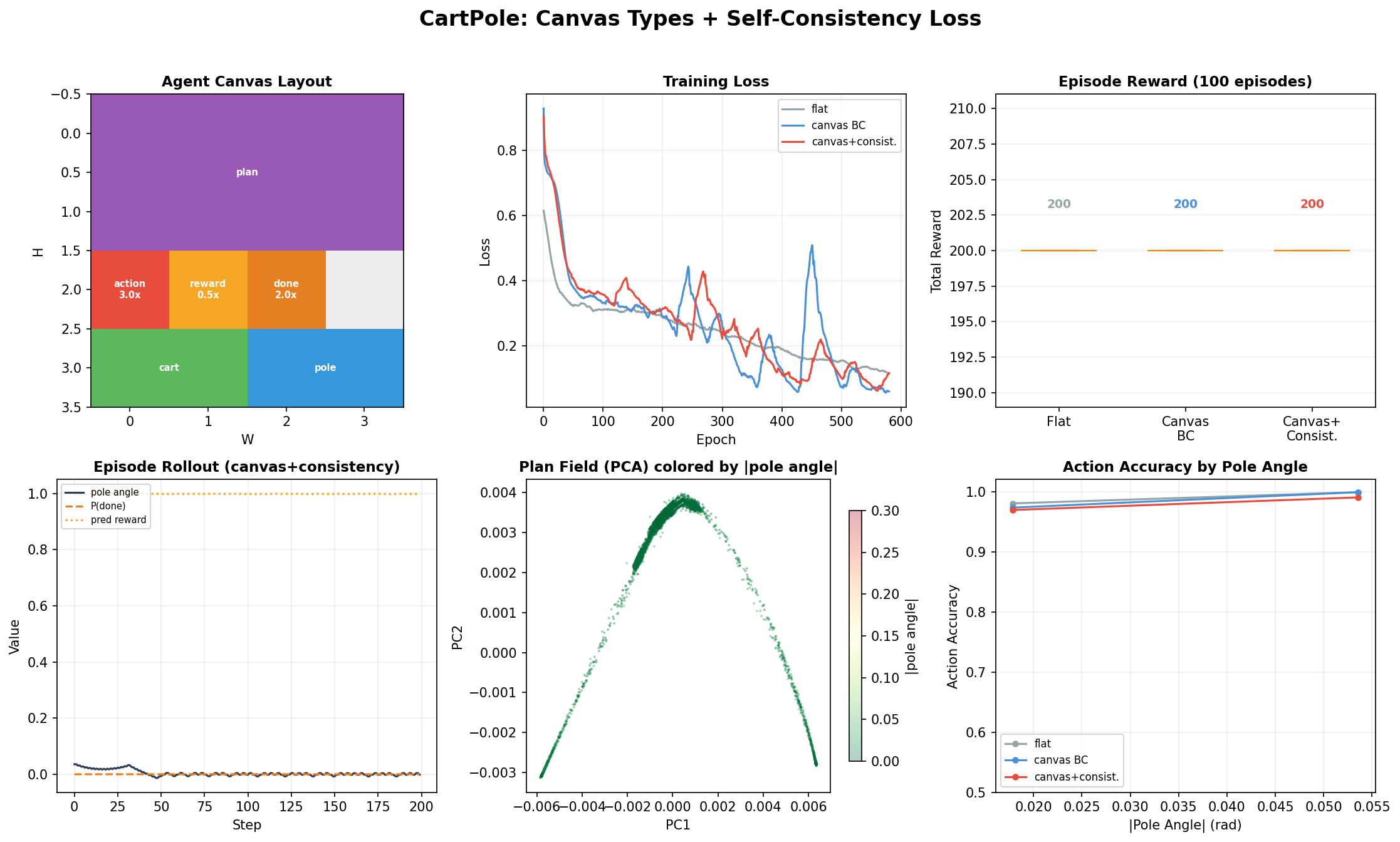
Top left: Agent canvas layout — observation split into cart (position, velocity) and pole (angle, angular velocity), a plan field with mamba attention for temporal reasoning, and separate action, reward, done output heads with different loss weights.

Top right: Training curves — the canvas+consistency model has higher total loss (it's optimizing more objectives) but produces richer internal representations.

Top center-right: Episode rewards — all three models achieve perfect 200 on CartPole (it's a solved environment), but the internal representations differ dramatically.

Bottom left: Single episode rollout showing the consistency model's predictions: pole angle tracks done probability (the consistency loss enforces this), and predicted reward inversely correlates with done.

Bottom center: Plan field PCA colored by pole angle — the most interesting panel. The plan field learns structured representations of the physical state without being told to. The PCA shows clear clustering by pole angle, meaning the latent planning state encodes task-relevant information purely from the type hierarchy and consistency loss.

Bottom right: Action accuracy by pole angle — all models are near-perfect, but accuracy matters most at large angles (near failure).

Type declaration

@dataclass
class Observation:
    cart: Field = Field(1, 2)      # position, velocity
    pole: Field = Field(1, 2)      # angle, angular velocity

@dataclass
class CartPoleAgent:
    obs: Observation = field(default_factory=Observation)
    plan: Field = Field(2, 4, attn="mamba")        # (1)
    action: Field = Field(1, 1, loss_weight=3.0)   # (2)
    reward: Field = Field(1, 1, loss_weight=0.5)   # (3)
    done: Field = Field(1, 1, loss_weight=2.0)     # (4)

1. plan: 8-position latent planning state with mamba attention (sequential temporal modeling). This field has no direct supervision — it learns useful representations from the gradients flowing through action, reward, and done.
2. action: 3× loss weight — this is the primary output we care about.
3. reward: 0.5× loss weight — auxiliary prediction, soft supervision.
4. done: 2× loss weight — predicting episode termination is safety-relevant.

The self-consistency loss

This is what makes this example more than SFT. The consistency loss enforces causal relationships between canvas fields:

if use_consistency:
    # Consistency 1: large pole angle -> high done probability
    pole_angle = obs[:, 2].abs()
    angle_signal = sigmoid(pole_angle * 10 - 2)
    consistency_angle = mse(done_prob, angle_signal)

    # Consistency 2: if done is high, reward should be low
    expected_reward = 1.0 - done_prob.detach()
    consistency_reward = mse(reward_pred, expected_reward)

    # Consistency 3: plan should be smooth (regularizer)
    plan_std = plan_field.std(dim=0).mean()
    consistency_plan = plan_std * 0.1

These are not labels — they're structural constraints between canvas fields. The model doesn't just predict actions; it builds an internal model where the reward, done, and observation predictions are mutually consistent.

This is canvas engineering

The type hierarchy (obs -> plan -> action/reward/done) declares the information flow. The connectivity policy wires it. The consistency loss enforces that the wiring carries meaningful information. Together, the plan field emerges as a compressed state representation — visible in the PCA plot — without any explicit representation learning objective.

Connectivity

bound = compile_schema(
    CartPoleAgent(), T=1, H=4, W=4, d_model=32,
    connectivity=ConnectivityPolicy(
        intra="dense",
        parent_child="hub_spoke",   # plan sees obs, action reads plan
    ),
)

hub_spoke means the agent-level fields (plan, action, reward, done) connect bidirectionally to all observation fields. This creates the information pathway: observation → plan → action/reward/done.

Expert data

500 episodes from a simple heuristic policy:

def expert_policy(obs):
    _, _, angle, ang_vel = obs
    return 1 if angle + ang_vel * 0.5 > 0 else 0

This achieves perfect 200-step episodes on CartPole-v1.

The three models

Model	Architecture	Training	What it learns
Flat	2-layer MLP	cross_entropy(action) only	Action mapping
Canvas BC	2-layer transformer on canvas	Action + reward + done	Multi-task on structured regions
Canvas + consistency	Same architecture	Action + reward + done + 3 consistency terms	Causally-grounded internal model

All three solve CartPole (it's too easy for a meaningful performance gap). The difference is in what they learn internally — the plan field PCA shows this clearly.

Run it

pip install gymnasium
python examples/03_cartpole_control.py
# Generates: assets/examples/03_cartpole.png

Takes ~30 seconds: 500 episodes of data collection, 600 epochs × 3 models, 100 evaluation episodes × 3.